The Memory Revolution in Artificial Neural Networks: The Technical Journey from RNNs to LSTMs
A detailed explanation of how recurrent connections and gating mechanisms function in neural networks to understand time-series data and human language.

In the field of Artificial Neural Networks, traditional feedforward neural networks process each input independently of one another. However, when working with sequential data such as text, audio, or time series, the order of the components becomes extremely important. To meet this need, Recurrent Neural Networks (RNN) were developed. An RNN maintains a type of internal memory by linking the output of its previous time step with the input of the current time step.
The fundamental component of an RNN is the recurrent unit, which possesses a hidden state. This hidden state acts as a memory that is continuously updated based on the current input and the previous hidden state. Mathematically speaking, an RNN is a function that processes an input vector xt and a hidden vector ht to yield a new output yt and a hidden vector ht+1 for the next time step. This feedback mechanism gives the model the power to learn from past inputs and apply that learning to current processing.
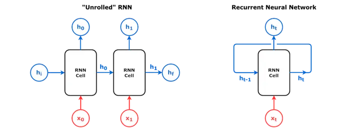
RNN-based models can be primarily divided into two parts: configurations and architectures. When various RNNs are connected in a data flow, it is called a configuration, and each RNN itself possesses a specific architecture. For deep processing, Stacked RNNs or deep RNNs are used, in which more than one RNN layer is arranged on top of another. Layer 1 receives the input x0,t and the hidden state h1,t to produce x1,t and a new hidden state h1,t+1, which acts as the input for the subsequent layer.
How RNN works: A step-by-step process
To understand the functioning of an RNN, it must be viewed unfolded in time across various temporal stages. At each time step, the model performs a series of computations using the same parameters and weights.
- Acceptance of input and hidden stateAt the current time step t, a new input xt and the hidden state ht-1 of the previous time step t-1 are received.
- Weighted calculation and transformationProcessed through a non-linear activation function by applying a weight matrix and bias to the input and the previous memory state.
- Update of hidden stateBased on the new calculation, the hidden state ht of the current time is updated, which acts as memory for the next time step.
- Output generationThe model proceeds by generating a specific prediction or result yt based on the current hidden state.
In the first stage, the network receives the data of the current time step and the memory of the past. In the second stage, it applies weights and bias to this information to perform a non-linear transformation. In the third stage, the hidden state is updated with the obtained result, and in the fourth stage, the output of that time step is generated.
The history from neuroscience and statistical mechanics to modern architectures
The roots of recurrent neural networks lie in neuroscience. In biology, the term "recurrent" is used for loop-like physical structures. In 1901, Cajal observed recurrent semicircles in the cerebellar cortex. Subsequently, in 1933, Lorente de Nó discovered recurrent connections and proposed that excitatory loops account for the vestibulo-ocular reflex. In the 1940s, a scientist named Hebb introduced the idea of a "reverberating circuit" to explain short-term memory. A 1943 paper by McCulloch and Pitts mentioned networks containing cycles, which could be influenced by past activities.
In 1960, Frank Rosenblatt published research on "closed-loop cross-coupled perceptrons." In 1961, he demonstrated that a fully cross-coupled perceptron network is equivalent to a feedforward network of infinite depth. Following this, similar networks were introduced by Kaoru Nakano in 1971, Shun'ichi Amari in 1972, and William A. Little in 1974. Statistical mechanics also made a major contribution to this field. The Ising model was developed by Wilhelm Lenz and Ernst Ising in the 1920s. In 1982, John Hopfield applied these principles to study the Hopfield network with a binary activation function and extended it to a continuous activation function in 1984.
વર્ષ
During the resurgence of neural networks in the 1980s, two important architectures emerged: the Jordan network by Michael I. Jordan in 1986 and the Elman network by Jeffrey Elman in 1990. Thereafter, in 1997, Mike Schuster and Kuldip K. Paliwal introduced bidirectional recurrent neural networks (BRNNs), which processed sequences in both forward and backward directions.
The Vanishing Gradient Problem and the Emergence of LSTM
When traditional RNN models are trained on long sequences, they face the vanishing gradient problem. When the model is trained via back-propagation through time, long-term gradients approach zero due to the multiplication of very small numbers. As a result, the model cannot remember information from the distant past and stops learning.
To overcome this severe limitation, the Long Short-Term Memory (LSTM) architecture was introduced in 1997 by Sepp Hochreiter and Jürgen Schmidhuber. LSTM provides a mechanism that allows gradients to flow for thousands of time steps without decaying. This enables the network to learn which information to remember for a long time and which information to forget.
For example, in Natural Language Processing, while processing the sentence "Dave, as a result of his controversial claims, is now a pariah", the LSTM model remembers the gender and number of the main subject 'Dave' so that proper grammar can be maintained with the subsequent pronoun 'his' and verb 'is'. After the verb 'is' appears, the model can understand that the need for that information is fulfilled and discard it.
Internal Architecture and Mathematical Equations of LSTM
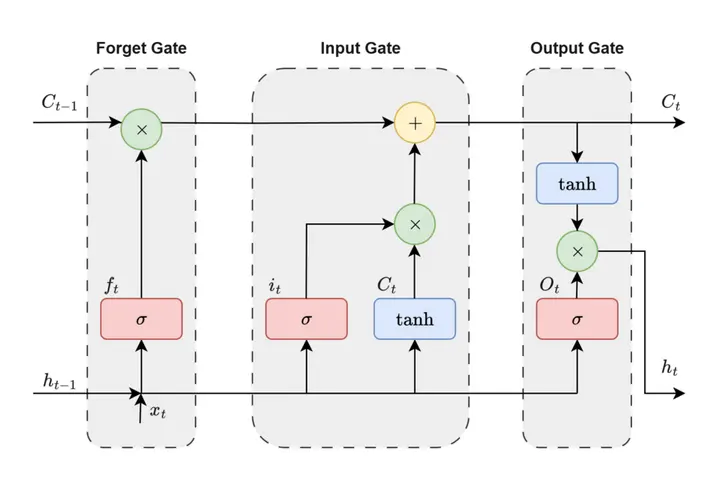
An LSTM unit is primarily composed of a memory cell and three gates: a forget gate, an input gate, and an output gate. These gates work to control the flow of information inside the cell.
The forget gate decides which information to remove from the previous state. It uses a sigmoid function to output a value between 0 and 1, where 0 means completely forgetting the information and 1 means completely remembering it. The input gate determines what new information to add to the cell state. The output gate controls what information from the current cell state should be outputted.
| Gate / Component | Mathematical Equation | Main Function |
|---|---|---|
| Forget Gate (ft) | ft = σg(Wf xt + Uf ht-1 + bf) | Determines which information to discard from the previous state (0 to 1) |
| Input Gate (it) | it = σg(Wi xt + Ui ht-1 + bi) | Determines what new information from the current input to store |
| Candidate State (~ct) | ~ct = σc(Wc xt + Uc ht-1 + bc) | Creates new candidate values to be added to the cell state |
| Cell State (ct) | ct = ft ⊙ ct-1 + it ⊙ ~ct | Updates the main state by forgetting old memory and adding new memory |
| Output Gate (ot) | ot = σg(Wo xt + Uo ht-1 + bo) | Determines which information from the cell state to send as output |
The vector equations for the forward pass of the computations taking place in an LSTM cell are as follows. Here σg denotes the sigmoid activation function and the ⊙ symbol denotes the Hadamard product (element-wise multiplication):
Forget gate: ft = σg(Wf xt + Uf ht-1 + bf) Input gate: it = σg(Wi xt + Ui ht-1 + bi) Output gate: ot = σg(Wo xt + Uo ht-1 + bo) Candidate cell state: c~t = σc(Wc xt + Uc ht-1 + bc) New cell state: ct = ft ⊙ ct-1 + it ⊙ c~t New hidden state: ht = ot ⊙ σh(ct)
Here the initial values are c0 = 0 and h0 = 0. The W and U matrices represent the weights of the input and recurrent connections respectively.
Advanced Applications, Bidirectional Models and the Transformer Era
In the mid-2000s, bidirectional architectures were combined with LSTMs. Bidirectional LSTM (Bi-LSTM) models yielded revolutionary results in the fields of speech recognition and text-to-speech, and were widely used in Google voice search. In 2010, Tomáš Mikolov and his colleagues showed that RNN-based language models yield better results than traditional n-gram models.

In 2014, Kyunghyun Cho and his team proposed the RNN encoder-decoder for machine translation. The same year, sequence-to-sequence learning was demonstrated using LSTM. This discovery played a foundational role in the development of attention mechanisms.
Later, more efficient alternatives such as the Gated Recurrent Unit (GRU) also emerged. In recent years, Transformer models based on self-attention have replaced RNNs in natural language processing because they excel in parallel processing. Even so, RNNs and LSTMs continue to play an important role today in devices where real-time processing and computational efficiency are extremely crucial.